Introduction to Effective Field Theories in Elementary and Collider Physics II: Applications

Office Hours and Infos

Homework Problems

• Interesting and useful homework problems will be identified and mentioned in class weekly.
• Let me know if you are interested in having a tutorial.

Lecture Notes and Exercises (Click here for the notes and the exercises of part I.)

• Lecture 6: Composite Operators and Effektive Weak Hamiltonian
  
  
  • Exercises (March 8, 2011): Strong Coupling Evolution (solutions and Mathematica notebook by Pedro Ruiz-Femenia)
    
    You should carry out the following exercises using Mathematica for some of the tedious algebra, but not blindly and still employing your brain for thinking what you are doing. The numerical values for the known coefficients of the QCD beta-function are as follows: 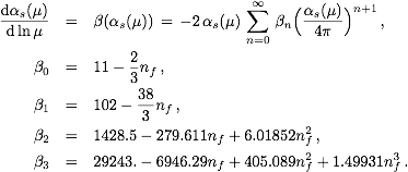For the numerical evaluations take n_f=5 and α_s(M_Z)=0.118 for M_Z=91.187 GeV as the initial condition for the solution.
    
    • (1) Strong coupling evolution (numerical): Solve the RGE for the strong coupling α_s. (a) Use the Mathematica routine NDSolve and program four little routines (or one single one) that determines α_s(μ) from α_s(μ₀), μ₀ and μ at one, two, three and four loop order.
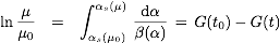
    • (2) Strong coupling evolution (analytical): There are plenty of methods for analytic solutions beyond the LL order, because contributions from higher orders can be treated differently. One method starts from the relation where and . Determine the coefficients of the function G(t) and then solve the equation iteratively for α_s(μ). This requires some careful thinking about what can be expanded in (and what not) and means that you start with a solution at the LL order level and determine the higher order contributions in a perturbative expansion. Note that all logarithmic dependence can be parametrized conveniently in terms of the expression 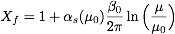. You have to keep the two terms in X_f together since they are both of order one. Plot the relative difference between the analytic and the purely numerical code at one, two, three and four loops as a function of μ.
    • (3) The hadronic scale &Lambda_QCD ("Lambda QCD"): Show that is a RG-invariant quantity. Analyze the expression at LL order. What is the physical interpretation of &Lambda_QCD? Determine &Lambda_QCD numerically at one, two, three and four loop order as a function of the renormalization scale μ.
    
    
  • Exercises (March 15, 2011): Large order behavior of perturbation theory: Renormalons (solutions by Maximilian Stahlhofen)
    
    The perturbative series of quantities computed in QCD (and in fact in essentially all quantum field theories) is not convergent. In QCD one reason for that is the behavior of quantum corrections related to the RG-evolution of the strong coupling.
    
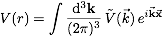
    • (1) Large order behavior of the static QCD (Coulomb) potential: In momentum space the leading order expression for the static QCD potential between a heavy quark and antiquark has the form . The dependence on the running coupling α_s at the momentum scale accounts for the summation of the most important higher order logarithmic terms. Take the running strong QCD coupling α_s at LL order, write the resulting series in powers of α_s(μ) and determine the configuration space static QCD potential by Fourier transformation, where .
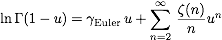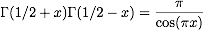
      The result can be determined with relatively little work using that powers of logarithms can be generated from derivatives of with respective to u. Rewrite the result in terms of gamma functions only, using the relation . Now rewrite the result in term of an exponential with the logarithm of the Gamma function and use the small u series expansion of logarithm of the Gamma function . Look up the properties of the zeta function ζ(n) for large n and then determine the asymptotic behavior of the perturbative coefficients in the &alpha_s series for the position space potential in the limit of large order n. Show that the coefficients diverge with n factorial, Γ(n+1)=n!. Series that have such a behavior are said to have a "Renormalon".
    • (2) Asymptotic series: What does this behaviour mean for the perturbative series? Do a little survey in the literature (or use Google) and find the criterion to show that the perturbative series is in fact an asymptotic series. Discuss during the tutorial about how such a series can have any physical meaning.
    • (3) IR Renormalon: Show that the bad n factorial behavior for the static configuration space potential at large orders of perturbation theory arises from small momenta k in the Fourier integration. The renormalon is therefore called an infrared-renormalon. One way to solve the exercise is to split the radial part of the Fourier integral into a low and a large momentum contribution. This exercise requires from you some over sight how to use mathematics in an efficient way.
    
    
    
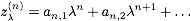
  • Exercises (March 23, 2011): (solutions by Pedro Ruiz-Femenia)
    
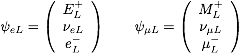
    • (1) Muon Decay: In the Fermi theory the amplitude for muon decay reads 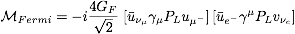where . Derive the Fermi constant G_F within the Standard Model and determine the muon decay width. You might set the electron mass to zero. Find the experimental muon width (from the PDG) and determine G_F (with experimental errors).
    • (2) An Alternative Model: Think back how the SM is constructed and which factors are relevant for the muon decay. What is the result for the Fermi constant in a theory in which the left-handed electron and muon fields are in triplets (with all right-handed fields in singlets) under as follows: , where E⁺ and M⁺ are heavy (unobserved) lepton fields? The SU(2) generators of the triplet representation are: . Note that .
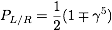
    • (3) Neutrino-Electron Elastic Scattering: In the theory, both W^+- and Z⁰ exchange contribute to the elastic scattering process . For momentum transfers very small compared to M_W, show that the amplitude for this process can be written as 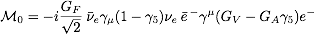. Find G_V and G_A.
    
    
  • Exercises (March 29, 2011): (solutions by Maximilian Stahlhofen)
    
    • (1) Fierz Transformation: Find the C_j in the following relations: . These six numbers are all there is to Fierz transformations. Hint: For (a) and (b), multiply by γ^ν_lk and sum over l and k. For (c) and (d), it's easiest to avoid taking traces of &sigma^μν, so multiply by δ_lk and sum over l and k to get one equation. Multiply by &delta_jk and sum over j and k to get another. To prove (b'), multiply by &gamma^λ_lk and sum over l and k.
    • (2) Mixing of 4-Quark Operators: Compute the mixing matrix Z^c_ij of the operators O₁ and O₂. Use color and Dirac Fierz relations discussed in class and recycle results obtained before for the one-loop renormalization of QED.
    
    
    
  • Exercises (April 5, 2011): (solutions by Maximilian Stahlhofen)
    
    • (1) Semileptonic and Nonleptonic B Decay Rates:
      a) Calculate the semileptonic decay rate of a free b quark . Use the effective Hamiltonian discussed in class. Write down the result for the muon decay rate.
      Now Use the effective Hamiltonian discussed in class to compute the non-leptonic free quark decay rate . Neglect all masses except for the b quark mass.
    • (2) Change of Renormalization Prescription: The MS subtraction scheme belongs to the class of ``mass-independent'' renormalization prescriptions. Another such scheme is the MS subtraction scheme where . So, consider the coupling in some theory defined in two mass-independent renormalization prescriptions, λ and λ. Their relation can be expressed in terms of a perturbative series, . Determine the coefficients a_i for the couplings in the MS (λ) and the The MS (λ ) schemes for the &phi⁴-theory. Prove that the first two coefficients of the β-functions in both schemes, are the same. Do the results also apply to QED and QCD?
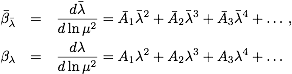
    • (3) Renormalization Group Equations at Higher Order:
      a) The renormalization constants of φ⁴-theory at two-loop order in the MS scheme read . Determine the two-loop renormalization group equations.
      Solve the renormalization group equations. To keep the solution elementary it can be helpful to recall that you anyway need to only consider the case λ<< 1. Coupling times log, however, is of order unity.
      b) Use the relation between the renormalized and the bare coupling, , to derive the general expression for in terms of Z_λ in d=4-2ε dimensions. Use the fact that does not diverge for ε→ 0 to show that the coefficient of the 1/ε² term in Z_λ can be determined from the coefficient of the 1/ε term. For this make the ansatz 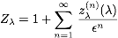. and use the fact that z_λ⁽ⁿ⁾ is of order λⁿ, i.e. . Cross-check the result with the two-loop result of Z_λ in φ⁴-theory. Explain that in fact all z_λ⁽ⁿ⁾ with n≥2 can be determined from z_λ⁽¹⁾. Derive the λ³/ε³ and λ³/&epsilon² three-loop contributions of Z_λ.
    
    
    
  • Exercises (April 10, 2011): (solutions by Pedro Ruiz-Femenia)
    
    • (1) Non-Leptonic b Quark Decays and Penguin Transitions:
      Write down all possible decays of a b quark into u, d, s and c quarks. (This includes decays into two or three of the same quarks.) Order the various decay modes into the following three classes:
      • Class I: only current-current operators contribute,
      • Class II: current-current and penguin operators contribute,
      • Class III: only penguin operators contribute.
      Determine the parametric size of the various operators (take into account matching conditions and CKM factors).
    • (2) The decay b → s γ and QCD Equations of Motion:
      After integrating out the top, W, Z and Higgs, a number of local operators are induced which mediate the flavor changing (electric) charge-neutral process b → sγ. The operators that are induced include the local 4-quark operators discussed in class and the following local 2-quark operators, which we, however, did not discuss in class: Here, D_μ=&part_μ + i g T^A A_μ^A + i e Q A_μ is the covariant derivative (in the SU(3) fundamental representation) acting on the quark fields, (D^μ G_μν)^A = (δ^AB ∂^μ + g f^ABCA^{μ B}) G_μν^C and .
      (a) Write down the combined QCD-QED Lagrangian (i.e. only operators up to dimension-4) and derive the equations of motion for the gluon and quark fields. Note that this is a classic problem. So, for the QED equations of motion remember your courses on electrodynamics. The QCD equations of motion are derived in an analogous way.
      (b) You can take the classic equations of motion for the dominant dimension-4 action to reduce the dimension-6 operators shown above to linear combinations of O₈ and O₉ and the 4-quark operators treated in class. One can in fact prove that this eliminates the 2-quark operators also at the quantum level. Take m_s=0, but keep the bottom quark mass nonzero. You will find the identity quite useful. For O₇ you need the identity with three gamma matrices .
  
  
  
• Lecture 7: Heavy Quark Effective Theory
  
  
  • Exercises (May 3, 2011): (solutions by Pedro Ruiz-Femenia)
    
    • (1) Heavy antiquarks in HQET: Recall how the HQET Feynman rules for the heavy quark were derived in class (propagator and single gluon interaction vertex). Now consider the corresponding Feynman rules for the heavy antiquark. Since in HQET the quark and antiquark dynamics is decoupled (because we do not have to care about covariance), we want to formulate the effective theory for heavy antiquarks having positive energy. In the limit, show that the propagator for a heavy antiquark with momentum p_Q = m_Q v+k is while the heavy antiquark-gluon vertex is . This exercise is not difficult, but it requires that you keep carefully track of color and Dirac indices, and that you know about charge conjugation and its meaning within the relativistically covariant formulation of quantum field theory (Stueckelberg interpretation).
      
      
    • (2) Operator Renormalizaton in HQET: Compute the MS wave function renormaliation constant of a heavy quark. Now recall the rules to do operator renormalization and determine the renormalization of the heavy-to-light current and the heavy-to-heavy current . Note that the heavy quark fields in the heavy-to-heavy current have different v-labels. So while we in general have . Recall that in HQET there are different v-sectors, each labelled with a different v and that the Feynman rules in each of these sectors depend on v, but look the same otherwise. These different v-sectors are coupled through the heavy-to-heavy currents.
      Determine the anomalous dimensions of the heavy-to-light and the heavy-to-heavy currents. Analyze the anomalous dimension of the heavy-to-heavy current for the limit and interpret the result physically.
    
    
    
  • Exercises (May 10, 2011): (solutions by Maximilian Stahlhofen)
    
    • (1) Anomalous dimension of c_F: Up to order 1/m_Q the HQET Lagrangian has the form . Derive the HQET Feynman rules at order 1/m_Q and draw the diagrams one needs to compute to determine the anomalous dimension of the coefficient c_F. Discuss at the level of the diagrams whether the 1/m_Q kinetic energy operator can mix with the magnetic moment operator. Write down the color structure of each of the diagrams contributing to the anomalous dimension of the c_F and argue that the anomalous dimension is proportional to the QCD color factor C_A=3. (At this point it is helpful to carefully look at the diagrams and to remember current conservation in QED.) You don't have to actually compute any of the loop integrals.
      
      
    • (2) Renormalization of HQET at order 1/m_Q²: In the paper hep-ph/9708306 by Bauer and Manohar the LL renormalization of the HQET Lagrangian up to order 1/m_Q² is carried out. This is actually a reading assignment which should encourage you to reproduce some of the results shown in the paper. The only tricky part of the paper is that it treats the time-ordered products of the 1/m_Q operators as individual operators. This is just a notational trick to formulate insertions of two 1/m_Q operators in the framework of a linear (!) renormalization group equation involving operators at order 1/m_Q².
      The Wilson coefficient of such a time-ordered product is just the product of the Wilson coefficients of the operators that appear in it. You might actually appreciate how nicely this simple notational this trick works in practice.
      (a) Find the renormalization group equation for c_F and solve it.
      (b) Reproduce Eq.(9) which relates the Darwin operator O_D to the operator O₁^hl using the gluon equation of motion. This eliminates the operator O₁^hl from the anomalous dimension matrix shown in Eq.(14). Derive the anomalous dimension matrix for the operator basis where O₁^hl is eliminated. Note that in this paper the anomalous dimension matrix for the operators and not for the Wilson coefficients is shown!
      (c) Find the solution for c_D and c_F using the matching conditions c_D(μ=m_Q) =c_S(μ=m_Q)=1.
    
    
    
  • Exercises (May 17, 2011): (solutions by Pedro Ruiz-Femenia)
    
    • (1) Heavy quark limit and the decays ( D₁, D₂^* ) → ( D, D^* ) + π : The members of the s_l=3/2 (spin of the light degrees of freedom) doublet ( D₁, D₂^*) can decay by means of a single pion emission into the two members of the s_l=1/2 ground state doublet (D, D^*). The decay it governed by the strong interaction. So in addition to parity and angular momentum conservation, also heavy quark spin symmetry can be applied in the limit m,sub>c,/sub>→∞. Parity restricts the orbital angular momentum L of the emitted pion (P(π)=-1). Determine the relative amplitudes and the relative decay partial widths for the four possible decays using a Clebsch-Gordan analysis in the heavy quark limit. You need to use the Wigner-Eckard theorem and heavy quark spin symmetry to obtain the expressions for each of the dominant possible partial waves L. Show among the first things that all non-zero transitions have a final state with orbital angular momentum L=2 as the dominant partial wave. Use parity and angular momentum conservation for the argumentation and recall that the heavy quark spin is conserved for the deday. The latter also leads to restrictions of the total spin of the light degrees of freedome. Only keep the dominant partial wave for going on.
      The largest source of heavy quark symmetry breaking arises from the fact that the charm mass is actually not really infinite. This leads to sizeable differences in the phase spaces available for the pion for the various decay channels. (Consult the PDG for the D meson and pion masses.) The phase space of the pion for partial wave L is to a good approximation proportional to |p_π|^2L+1 in the (D₁, D₂^*) rest frame, p_π being the pion momentum. Include the corrections arising from this effect into the relative size of the four decay rates and compare to the experimental numbers in the PDG.
      Compare the previous experimental numbers to those for the analogous decays of the s_l=1/2 doublet (D₀*, D₁*) into the ground state doublet plus a pion which have been seen. Explain the difference. (You only need to compare the overall size of the rates and shall not carry out the same analysis you did for the ( D₁, D₂^* ) decays.
    
    
    
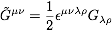
  • Exercises (May 24, 2011): (solutions by Maximilian Stahlhofen)
    
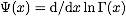
    • Non-relativistic Schroedinger Equation : The non-relativistic Schr\"odinger equation for the positronium has the form 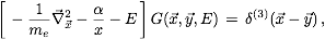, where α is the fine structure constant, m_e the electron mass and E the energy of the electron-positron system with respect to 2m_e. G is the Green function.
      (a) Show that with β=(E/m_e)^1/2, is a solution of the Schroedinger equation for .
      (b) Compute the integral for G(r,0,E) in terms of appropriate special functions and determine limit r → 0. What do the divergences mean? Show that these divergences lead to infinities in time-independent perturbation theory. (Consider the corrections caused by the Darwin potential ).
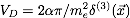      (For this exercise you should/must consult function and integral tables such as Gradstheyn-Ryzhik to find out about the integrals and the properties of the special functions that result from the integrals!!!!. The result has the form , where the Ψ-function is .)
      (c) G^r(0,0,E) (or better the expression obtained in the limit G(r→ 0,0,E)) has poles at the positronium bound state energies E_n. Determine the Coulomb spectrum and the positronium masses and determine the residue for E → E_n. What is the physical meaning of the residue?
      (d) Determine the Schroedinger equation for the Green function in momentum space. Note that 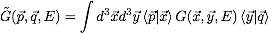where .
      [The solution has the form .]
      (e) Construct the Green function in momentum space perturbatively (i.e. iteratively) for small α to all orders and compute G^{dim. reg.}(0,0,E) using dimensional regularization in n=3-2ε dimension in the limit ε→ 0. For the two-loop diagram you can use the result . For the one-loop diagram you can use the results we already obtained in previous exercises (see also EFT lecture I). For the sum of three and more loop diagrams you can use the expression obtained in (b). (Why?)
      (f) (Exercise to be demonstrated by the tutor: Show that one can obtain the integrand of the two-loop diagram from expanding the electron-positron elastic scattering amplitude with the exchange of one photon in the t-channel in the nonrelativistic limit.)
      (g) Determine the imaginary part of G(0,0,E) for positive and negative energies. Show that in the continuum, for electron-positron scattering with positive energies, one recovers the famous Sommerfeld factor 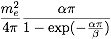. Where does this factor play a role? (See e.g. Landau/Lifschitz.)

  ---

  Maximal Syllabus (we will not cover all of the items)

  • Introductory Part (WS 2010/2011)
    • Review of the Standard Model
    • Standard Model as part of an effective theory.
  • Renormalization and Loops, Part I (WS 2010/2011)
  • Decoupling (WS 2010/2011),
    • EFT for QED with massive fermions (WS 2010/2011),
    • EFT for the Standard Model for heavy top, W, Z
    • Unification of gauge couplings (WS 2010/2011)
  • Renormalization and Loops, Part II: mixing,
  • General Aspects of QCD (WS 2010/2011)
  • Behavior of High-Order Perturbation Theory
    • Power Corrections
    • Renormalons
  • Heavy-Quark-Effective Theory
    • Symmetries, Action, Power Counting
    • Form Factors, CKM Matrix Elements
    • Radiative Corrections, Renormalization
    • Non-perturbative Corrections
    • Inclusive, Semileptonic Decays
  • Non-relativistic QCD
    • Degrees of Freedom, Action, Velocity Power Counting
    • Derivation of the Nonrelativistic Schroedinger Equation
    • Lamb-Shift
  • Chiral Perturbation Theory
    • Chiral Symmetry, Anomalies, Power Counting
    • Electromagnetic Processes
    • Pion, Kaon Processes
  • QCD Factorization, Soft Collinear Effective Theory
    • Collinear Fields and Operators, Symmetries, Power Counting
    • Factorization
    • Deep Inelastic Scattering
    • B Decays into light Hadrons
    • Aspects of Jet Physics

  ---